
Comparing Dependent Variable Model Transformations by Leave-one-out Cross-Validation in R
This article was originally published on Towards Data Science: Link
Optimising the predictive power of linear regression models by transforming the dependent variable and utilising cross-validation.
When deciding on a dependent variable transformation to enable optimal predictive power, a key concern is that the R-squared values (which are commonly used to measure the predictive fit of different models) are no longer comparable. Since R-squared is the proportion of the variance in the dependent variable that is explained by the variation in the independent variables, by performing transformations on the dependent variable we have also transformed their variance structures. As such, we can no longer gain insight into the relative predictive power of the different models by comparing their R-squared values.
Box-Cox Power Transformations
Although one may use the Box-Cox power transformation to get an indication of which transformation will help our model fit the data, this method will not help us with a measure of how well the transformed model performs for prediction, nor will it indicate whether using the mean or median predictor when rewinding the transformation will yield the best predictions. The following example highlights the issue relying too heavily on the Box-Cox transformation alone by employing leave-one-out cross-validation to calculate a comparable predictive power measure.
Leave-one-out Cross-validation
Cross-validation can be used as a means to enable comparison of the different dependent variable transformations. The leave-one-out method of cross-validation uses one observation from the sample data set to be used as the validation data, using the remaining observations as training data. Each model is used to predict the value of the validation data point by fitting the training data, then a prediction error is calculated by subtracting the predicted value from the validation data observation. To ensure we obtain comparable measures, it is essential that the fitted value produced by the transformed models are converted back to the “level” form to obtain a predicted value that is in the same units as the original observation data. Using different methods for this conversion enables the comparison of the mean and median predictors. This process is repeated, until each observation from the original sample has been used as a validation data point, then by summing the absolute values* of the prediction errors we obtain a measure of how well the transformed model in question makes out-of-sample predictions. Once the cross-validation measure has been calculated for each transformation (and applicable predictor type), the model that produces the lowest measure is deemed to have the greatest predictive power.
‘One may instead wish to use the sum of squares of the prediction errors to calculate the comparison.
Worked Example
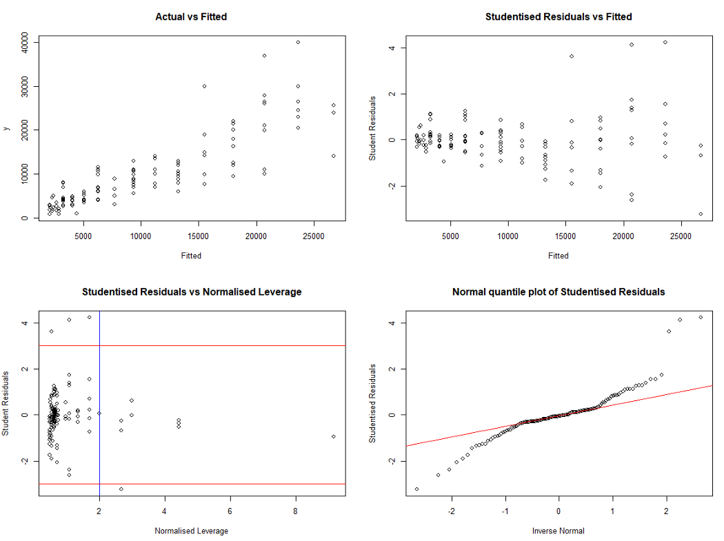
With the attached mazda.csv data set we wish to develop a model that will predict the price of a car, given its age. Following initial observations, it is determined that the inclusion of an age-squared term as a second variable in the model will help to alleviate non-linearity concerns. The below diagnostic plots are then produced.
Model: \(Price = α + β*Age + δ*Age²\)
# LOAD & ORGANISE DATA #####################################
original_data <- rio::import("mazda.csv")
data <- original_data
names(data) <- c("Year", "y", "x")
# Inclusion of Age^2 variable
x_sq <- data$x^2
data <- tibble::add_column(data, x_sq, .after = 100)
# MODEL DEVELOPMENT ########################################
reg1 <- glm(y ~ x + x_sq,
data = data)
fitted.1 <- stats::fitted(reg1)
resid.1 <- stats::resid(reg1)
stu.resid.1 <- MASS::studres(reg1)
leverage.1 <- sur::leverage(reg1)
norm_lev.1 <- (nrow(data)*leverage.1)/(length(coef(reg1)))
# Diagnostic Plots
par(mfrow = c(2, 2))
plot(fitted.1, data$y, main = "Actual vs Fitted", ylab = "y", xlab = "Fitted")
plot(fitted.1, stu.resid.1, main = "Studentised Residuals vs Fitted", ylab = "Student Residuals", xlab = "Fitted")
plot(norm_lev.1, stu.resid.1, main = "Studentised Residuals vs Normalised Leverage", ylab = "Student Residuals", xlab = "Normalised Leverage")
abline(v=2, col="blue")
abline(h=3, col="red")
abline(h=-3, col="red")
qqnorm(stu.resid.1, , main = "Normal quantile plot of Studentised Residuals",
xlab = "Inverse Normal", ylab = "Studentised Residuals",
plot.it = TRUE, datax = FALSE,)
qqline(stu.resid.1 , col="red")
par(mfrow=c(1, 1))
Although the inclusion of this term has helped linearise the diagnostics graphs, we are left with 2 concerns, namely the increasing variance for larger fitted values (heteroskedasticity) and non-normal residuals. We know that both of these issues can be addressed by transforming the dependent variable, and perform a Box-Cox power transformation to see which type of dependent variable transformation may be suitable.
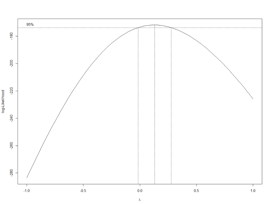
The Box-Cox Power transformation graph above suggests that transforming our Price variable by a log transformation would be suitable (since 0 lies within the 95% confidence interval of lambda, λ). However we know that a square-root transformation can also help alleviate the heteroskedasticity and achieve residuals that more closely follow a normal distribution. Therefore we decide to test both a log transformation and a square-root transformation of Price (as well as our initial linear model as a control) using leave-one-out cross-validation to determine which model will likely produce the best out-of-sample fit.
# BOX-COX TRANSFORMATION ###################################
box_cox <- MASS::boxcox(reg1, optimise = T, lambda = seq(-1,1, by=.1), main = "Box-Cox Power Transformation")
lamda_bc <- box_cox$x[which.max(box_cox$y)]
roundlamda_bc <- plyr::round_any(lamda_bc, .5)
# We see the Box-Cox transformation suggests a Log-transformation is most appropriate
# However lamda is close enough to 0.5 to also consider a square-root transformation.
Using the accompanying R script, we perform the LOO cross-validation for the three models. To ensure comparability of our cross-validation measure, we must convert out predicted values back to their “level” value before comparing them to the original observations being used as the validation data. Here we can choose either the mean or median predictor. For the model where no transformation is made, the mean and median predictors will be the same, however for the log and square-root models they are not. Therefore we can test these also via cross-validation to see which predictor obtains the lowest cross-validation measure by use of the below formulas when converting our fitted values back to the “level” prediction value. The accompanying R script performs each of these conversions within the respective cross-validation loop in calculating the comparable predictive power measures.
Log transformation:
- Mean Predictor: \((log) = exp(fitted)*exp(1/2*MSE)\)
- Median Predictor: \((log) = exp(fitted)\)
Square-root transformation:
- Mean Predictor: \((sqrt) = (fitted)² + MSE\)
- Median Predictor: \((sqrt) = (fitted)²\)
‘where ‘fitted’ is our predicted value and ‘MSE’ is the mean-squared error of the model.
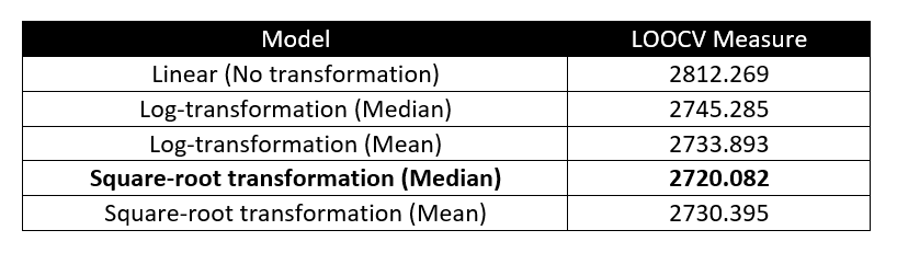
Thus we can compare the calculated measures to see which model and predictor performs best in terms of cross-validation. From the below table, we see that it is in fact the square-root transformed model that performs best in terms of cross-validation, with the median predictor obtaining the lowest LOOCV measure.
# LEAVE-ONE-OUT CV #########################################
dep.cv.glm <- function(x, data, mean.pred = TRUE, trans = "no"){
if(trans == "no"){
devn.1 <- list()
for(i in 1:nrow(data)) {
reg1.cv <- glm(formula(x),
data = dplyr::slice(data,-i))
fitted.cv1 <- predict(reg1.cv, newdata = data)
devn.1[i] <- ((data$y[i])-(fitted.cv1[i]))
}
devn.1 <- as.numeric(devn.1)
devn.1 <- abs(devn.1)
cv.lin <- mean(devn.1)
cv.lin
}
else if((mean.pred == TRUE) & (trans == "log")){
devn.1 <- list()
for(i in 1:nrow(data)) {
reg1l.cv <- glm(formula(x),
data = dplyr::slice(data,-i))
logfitted.cv1l <- predict(reg1l.cv, newdata = data)
mse <- summary(reg1l.cv)$dispersion
fitted.cv1l <- exp(logfitted.cv1l)*exp(0.5*mse)
devn.1[i] <- ((data$y[i])-(fitted.cv1l[i]))
}
devn.1 <- as.numeric(devn.1)
devn.1 <- abs(devn.1)
cv.log.mean <- mean(devn.1)
cv.log.mean
}
else if((mean.pred == FALSE) & (trans == "log")){
devn.1 <- list()
for(i in 1:nrow(data)) {
reg1l.cv <- glm(formula(x),
data = dplyr::slice(data,-i))
logfitted.cv1l <- predict(reg1l.cv, newdata = data)
mse <- summary(reg1l.cv)$dispersion
fitted.cv1l <- exp(logfitted.cv1l)
devn.1[i] <- ((data$y[i])-(fitted.cv1l[i]))
}
devn.1 <- as.numeric(devn.1)
devn.1 <- abs(devn.1)
cv.log.mean <- mean(devn.1)
cv.log.mean
}
else if((mean.pred == TRUE) & (trans == "sqrt")){
devn.1 <- list()
for(i in 1:nrow(data)) {
reg1s.cv <- glm(sqrt(y) ~ x + x_sq,
data = dplyr::slice(data,-i))
sqrtfitted.cv1s <- predict(reg1s.cv, newdata = data)
mse <- summary(reg1s.cv)$dispersion
fitted.cv1s <- ((sqrtfitted.cv1s)^2)+mse
devn.1[i] <- ((data$y[i])-(fitted.cv1s[i]))
}
devn.1 <- as.numeric(devn.1)
devn.1 <- abs(devn.1)
cv.sqrt.mean <- mean(devn.1)
cv.sqrt.mean
}
else if((mean.pred == FALSE) & (trans == "sqrt")){
devn.1 <- list()
for(i in 1:nrow(data)) {
reg1s.cv <- glm(sqrt(y) ~ x + x_sq,
data = dplyr::slice(data,-i))
sqrtfitted.cv1s <- predict(reg1s.cv, newdata = data)
mse <- summary(reg1s.cv)$dispersion
fitted.cv1s <- ((sqrtfitted.cv1s)^2)
devn.1[i] <- ((data$y[i])-(fitted.cv1s[i]))
}
devn.1 <- as.numeric(devn.1)
devn.1 <- abs(devn.1)
cv.sqrt.median <- mean(devn.1)
cv.sqrt.median
}
}
# RESULTS ##################################################
MSE.LOO.cv <- list()
MSE.LOO.cv[1] <- dep.cv.glm(y ~ x + x_sq, data, mean.pred = TRUE, trans = "no")
MSE.LOO.cv[2] <- dep.cv.glm(log(y) ~ x + x_sq, data, mean.pred = FALSE, trans = "log")
MSE.LOO.cv[3] <- dep.cv.glm(log(y) ~ x + x_sq, data, mean.pred = TRUE, trans = "log")
MSE.LOO.cv[4] <- dep.cv.glm(sqrt(y) ~ x + x_sq, data, mean.pred = FALSE, trans = "sqrt")
MSE.LOO.cv[5] <- dep.cv.glm(sqrt(y) ~ x + x_sq, data, mean.pred = TRUE, trans = "sqrt")
names(MSE.LOO.cv) <- c("Linear", "Log-Median", "Log-Mean", "Sqrt-Median", "Sqrt-Mean")
MSE.LOO.cv
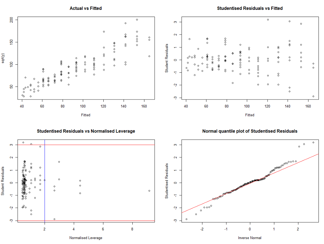
Taking a final look at the diagnostics plot of the preferred model we can see that the square-root transformation has significantly alleviated our concerns regarding heteroskedasticity and non-normal residuals. As such we can use the square-root transformed model and median predictor to produce predictions and prediction intervals relatively comfortably.
Model: \(sqrt(Price) = α + β*Age + δ*Age²\)
# PREFERRED MODEL ##################################################
reg1 <- glm(sqrt(y) ~ x + x_sq,
data = data)
fitted.1 <- stats::fitted(reg1)
resid.1 <- stats::resid(reg1)
stu.resid.1 <- MASS::studres(reg1)
leverage.1 <- sur::leverage(reg1)
norm_lev.1 <- (nrow(data)*leverage.1)/(length(coef(reg1)))
# Diagnostic Plots (Preferred Model)
par(mfrow = c(2, 2))
plot(fitted.1, sqrt(data$y), main = "Actual vs Fitted", ylab = "sqrt(y)", xlab = "Fitted")
plot(fitted.1, stu.resid.1, main = "Studentised Residuals vs Fitted", ylab = "Student Residuals", xlab = "Fitted")
plot(norm_lev.1, stu.resid.1, main = "Studentised Residuals vs Normalised Leverage", ylab = "Student Residuals", xlab = "Normalised Leverage")
abline(v=2, col="blue")
abline(h=3, col="red")
abline(h=-3, col="red")
qqnorm(stu.resid.1, , main = "Normal quantile plot of Studentised Residuals",
xlab = "Inverse Normal", ylab = "Studentised Residuals",
plot.it = TRUE, datax = FALSE,)
qqline(stu.resid.1 , col="red")
par(mfrow=c(1, 1))
Conclusion
This guide has outlined why comparing R-squared valued is not valid when comparing models with the different transformation of the dependent variable. The guide suggests that the use of a Box-Cox power transformation can help identify suitable transformations of the dependent variable, however, the Box-Cox transformation alone will not ensure our model performs optimally when making out-of-sample predictions. This guide and attached R script will enable users to perform leave-one-out cross-validation to test and compare the predictive power of models with different transformations of the dependent variable, and indicate whether the mean or median predictor is most appropriate.
Thanks for reading all the way to the end of the article! I’d love to hear any comments about the above. Feel free to leave a message, or reach out to me through LinkedIn.
Attachment A — Mazda.csv data file: Link
Attachment B — R Package List
# Packages #############################
pacman::p_load(pacman, dplyr, MASS, plyr, rio, tidyverse)